Supervised Learning Algorithms:
Linear Regression :
import numpy as np
import matplotlib.pyplot as plt
from sklearn.linear_model import LinearRegression
# Input data
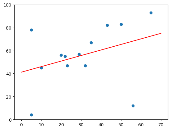
time_studied = np.array([20, 50, 32, 65, 23, 43, 10, 5, 22, 35, 29, 5, 56]).reshape(-1, 1)
scores = np.array([56, 83, 47, 93, 47, 82, 45, 78, 55, 67, 57, 4, 12]).reshape(-1, 1)
# Create and train the model
model = LinearRegression()
model.fit(time_studied, scores)
# Predict the score for a specific value
print(model.predict(np.array([56]).reshape(-1,1)))
# Plotting
plt.scatter(time_studied, scores)
plt.plot(np.linspace(0, 70, 100).reshape(-1, 1), model.predict(np.linspace(0, 70, 100).reshape(-1, 1)), 'r')
plt.ylim(0, 100)
plt.show()Note : The
LinearRegressionmodel expects input in a 2D array format for prediction.
Explanation :
np.linspace(0, 70, 100):- Function: Generates 100 evenly spaced values between 0 and 70.
.reshape(-1, 1):- Function: Reshapes the 1D array into a 2D array with 100 rows and 1 column.
model.predict(...):- Function: Uses the trained
LinearRegressionmodel to predict the scores for the generated values.
- Function: Uses the trained
plt.plot(..., ..., 'r'):- Function: Plots the input values against the predicted scores.
- First Argument: The x-values for the plot, which are the evenly spaced values between 0 and 70.
- Second Argument: The y-values for the plot, which are the predicted scores.
- Third Argument (
'r'): Specifies the color and style of the plot line.'r'means a red line.
Output :
[[68.22055244]]
Testing :
import numpy as np
import matplotlib.pyplot as plt
from sklearn. linear_model import LinearRegression
from sklearn.model_selection import train_test_split

# Input data
time_studied = np.array([20, 50, 32, 65, 23, 43, 10, 5, 22, 35, 29, 5, 56]).reshape(-1, 1)
scores = np.array([56, 83, 47, 93, 47, 82, 45, 78, 55, 67, 57, 4, 12]).reshape(-1, 1)

# randomly split both np array into 70% , 30%
# as test_size = 0.3 which means 30%
time_train, time_test, score_train, score_test = train_test_split(time_studied, scores, test_size = 0.3)

model = LinearRegression()
model.fit(time_train, score_train)

# Printing accuray
print(model.score(time_test, score_test))

plt.scatter(time_train, score_train)
plt.plot(np.linspace(0,70,100).reshape(-1,1), model.predict(np.linspace(0,70,100).reshape(-1,1)), 'r')
plt.show()
Logistic Regression :
import numpy as np
import matplotlib.pyplot as plt
from sklearn.model_selection import train_test_split
from sklearn.linear_model import LogisticRegression
# Example data
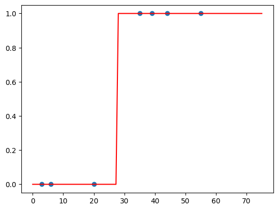
X = np.array([20, 10, 3, 6, 39, 43, 55, 44, 75, 35]).reshape(-1, 1)
y = np.array([0, 0, 0, 0, 1, 1, 1, 1, 1, 1])
# Split the data into training and test sets
X_train, X_test, y_train, y_test = train_test_split(X, y, test_size=0.3, random_state=42)
# Initialize and train the logistic regression model
model = LogisticRegression()
model.fit(X_train, y_train)
# Print accuracy
print(model.score(X_test, y_test))
# Predict on new data
new_data = np.array([22, 9]).reshape(-1, 1)
predictions = model.predict(new_data)
print(f"Predictions for new data: {predictions}")
# Plotting
plt.scatter(X_train, y_train)
plt.plot(np.linspace(0, 75, 100).reshape(-1, 1), model.predict(np.linspace(0, 75, 100).reshape(-1, 1)), 'r')
plt.show()
NOTE : the target array
yshould be a 1D array rather than a 2D column vector when passed to thefitmethod ofLogisticRegression
NOTE :
random_stateis an fixed state of when shuffled so u get same accuracy for samerandom_state
OUTPUT :
1.0
Predictions for new data: [0 0]
K-Nearest Neighbors (KNN) :
from sklearn.datasets import load_breast_cancer
from sklearn.neighbors import KNeighborsClassifier
from sklearn.model_selection import train_test_split
import numpy as np

data = load_breast_cancer()

print(data.feature_names)
print(data.target_names)
# print(data.data)
# print(data.target)

x_train, x_test, y_train, y_test = train_test_split(np.array(data.data), np.array (data.target), test_size=0.2, random_state=42)

clf = KNeighborsClassifier(n_neighbors=3)
clf.fit(x_train, y_train)
print(clf.score(x_test, y_test))
NOTE : K-Nearest Neighbors algo checks nearest K number of points in graph and then predict the group/cluster/class of unknown value.
n_neighbors = 3 means it checks for 3 neighbors for unknown points.
OUTPUT :
['mean radius' 'mean texture' 'mean perimeter' 'mean area' 'mean smoothness' 'mean compactness' 'mean concavity' 'mean concave points' 'mean symmetry' 'mean fractal dimension' 'radius error' 'texture error' 'perimeter error' 'area error' 'smoothness error' 'compactness error' 'concavity error' 'concave points error' 'symmetry error' 'fractal dimension error' 'worst radius' 'worst texture' 'worst perimeter' 'worst area' 'worst smoothness' 'worst compactness' 'worst concavity' 'worst concave points' 'worst symmetry' 'worst fractal dimension']
['malignant' 'benign']
0.9298245614035088
Support Vector Machines (SVM) :
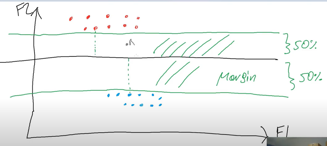
Assume we have 2 features (F1 and F2) and 2 groups (red and blue) of data SVM uses vectors and find a line (as in above example we have a 2D graph)
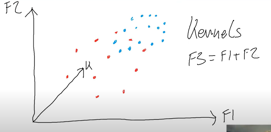
Assume we have only 2 features but as shown above data is clearly unseparable So we make a new feature using F1 and F2 called Kernel So now as we have 3D space graph we will find a ’ PLANE ’
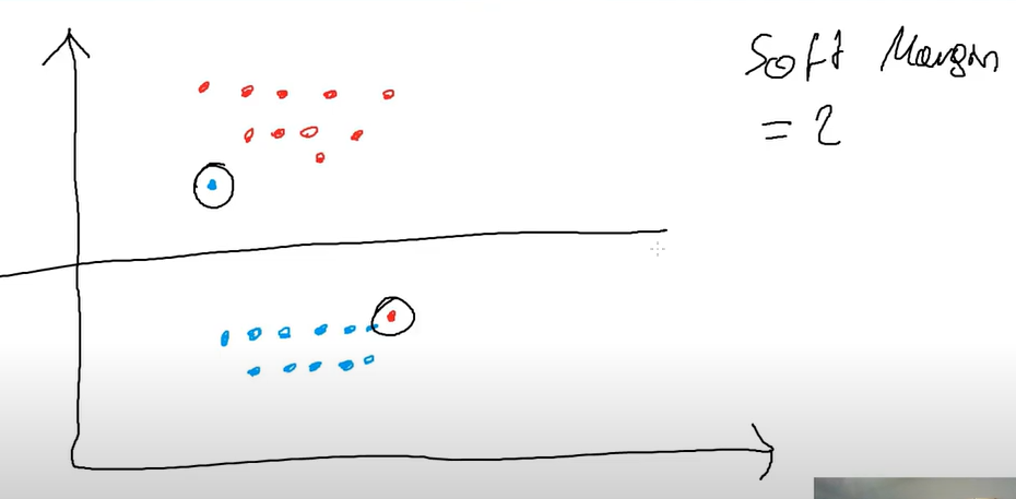
Soft Margin : we allow some imperfections in our data like above we set soft margin of 2 allowing both circled imperfect data to be ignored.
from sklearn.datasets import load_breast_cancer
from sklearn.model_selection import train_test_split
from sklearn.svm import SVC

data = load_breast_cancer()
X = data.data
Y = data.target

x_train, x_test, y_train, y_test = train_test_split(X, Y, test_size=0.2)

clf = SVC(kernel='linear', C=3) # C is soft margin
clf.fit(x_train, y_train)

print(clf.score(x_test, y_test))
Here C == soft margin