Resources:
- Sutton & Barto Reinforcement Learning: An Introduction (2nd ed)
- Complete Deep RL course by UC Berkeley: CS285 Berkeley (Sergey Levine lectures)
- RL part of Hands On ML by Oreilly
- DeepMind x UCL | Introduction to Reinforcement Learning 2015
Model Algorithms used in RL in brief
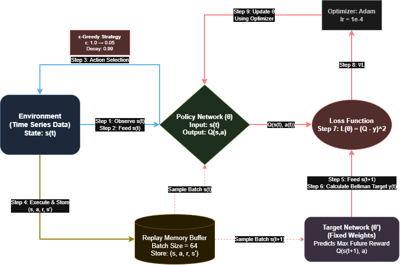
Value based Approximation (DQN) High Level View
The neural network takes the current state as input and outputs the expected cumulative future reward for each possible action at that state.
At time t and model parameters θ (weights and biasis):
- Observe state s(t)
- Feed s(t) to model get array of expected cumulative future rewards for each possible action { a(i)‘s } at that state. { Qθ(s(t), a(i))‘s }
- Choose action a(t) = action that has maximum future reward { argmax( Qθ(s(t),a(i)) ) }
- Execute the chosen action to which environment responds with (s(t+1), r(t))
- Feed s(t+1) to model get array of expected cumulative future rewards for each possible action { a(i)‘s } at that state. { Qθ(s(t+1), a(i))‘s }
- then we calculate Bellman target i.e. y(t) = r(t) + γ * max( Qθ(s(t+1),a(i)) )
- Loss i.e. L(θ) = ( Qθ(s(t), a(t)) - y(t) )
- Gradient of Loss w.r.t to current parameters (θ) i.e. ∇θL(θ)= 2 * ( Qθ(s(t),a(t)) − y(t) ) * ∇θQθ(s(t),a(t))
- For z(k) = w(k)^T * h(n−1) + b(k) neuron apply any optimizer
∂L / ∂z(k) = 2 * ( Qθ(s(t),a(t)) − y(t) )
In 4th and 5th step above, we use Relay Buffer and Target Network in actual implementation.
Policy-Based Approximation (REINFORCE as policy is softmax) High Level View
At time t and model parameters θ (weights and biasis):
- Observe state s(t)
- Feed s(t) to model get array of logits i.e. z
- Define a policy (πθ) lets say softmax i.e. πθ(a(i)∣s(t)) = e^z(i) / ∑e^z(i)
- Choose action i.e. a(t) ~ πθ(a(i)∣s(t))
- Execute the chosen action to which environment responds with (s(t+1), r(t))
- Store { s(t), a(t), r(t) }
After the episode ends at some t+n time:
- Compute return i.e. G(t) = r(t) + γ * r(t+1) + γ^2 * r(t+2) + …
- Policy Loss i.e. L(θ) = -[t=0 to t=n ∑logπθ(a(t)∣s(t)) ⋅ G(t)]
- Policy Gradient i.e. ∇θJ(θ) = -[t=0 to t=n ∑ ∇θlogπθ(a(t)∣s(t)) ⋅ G(t) ]
- Backprop through the policy network
- Optimizer update
Introduction:
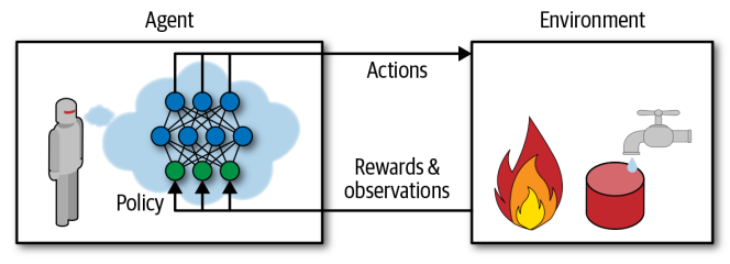
What is RL ?
- Mathematical formalism of learning-based decision making OR
- Approach for learning, decision making and control from experience.
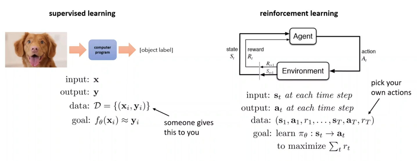
Supervised (standard) ML assumes:
- i.i.d data
- known outputs(ground truth) in training
RL assumes:
- data is not Independent and Identically Distributed (i.i.d) i.e. previous outputs influence future inputs.
- output(ground truth) is not known, only known if we succeeded or failed
- we know the reward
Data Driven AI (data):
- learns from real world data
- doesn’t try to do better than real world data
RL (optimization):
- optimize a goal with emergent behavior
- but need to figure out how to do that at scale
Deep RL (optimization at scale)
- learning from imitating (supervised learning iff i.i.d holds)
- so for a autonomous car, if the action taken causes the state to change such that it wasn’t in training(like going out of the lanes) then this causes the decision system to predict states that are off from expected next state
- we can solve this iff
- we cover all states (i.e. dataset is big and system has enough states)
- how we collect data
- change the algorithm / policy that decision system uses to take action
- learning from observing the data (unsupervised learning)
- transferring knowledge between domains (transfer learning, meta-learning)
- learning reward function from the world (RL)
- learning reward function from examples (inverse RL)
Supervised Learning: (x, y) → learn f: x → y Unsupervised Learning: (x) → learn structure of x Reinforcement Learning: (s, a, r, s’) → learn π: s → a that maximizes Σr
Policy Search
algorithm that agent / decision system uses to determine it’s actions
policy can be any algorithm, deterministic, non-deterministic etc.
policy space → all possible policies stochastic policy → random change in action policy search → tweak policy parameters
can use genetic algorithm to find for optimal policy i.e. randomly create n policies run all of them, kill x% of worst policies (leave some for diversity) and generate new policies by mutating (parent + random mutation) leftovers for next generation of policies.
policy gradients → tweak policy parameters to follow gradient of rewards with respect to policy parameters
Markov Decision Processes Framework
Markov Property → future is independent of past given present. Markov chains → stochastic processes(randomly evolves from one state to another at each step) with no memory.
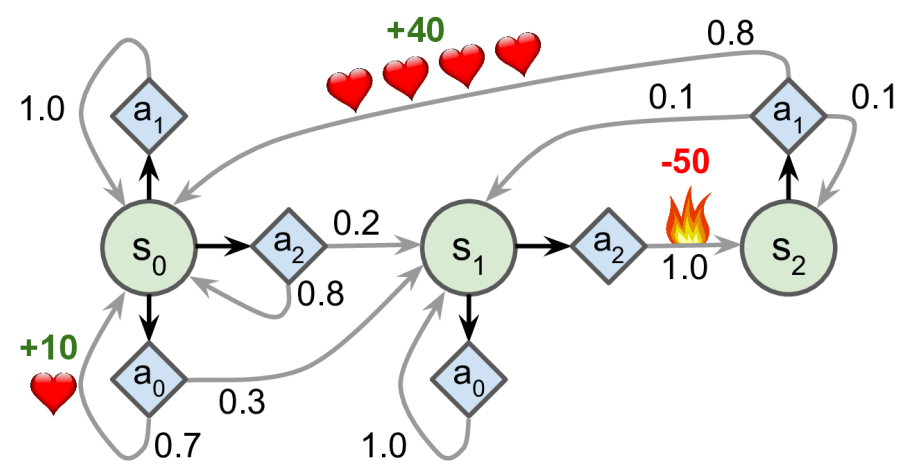 above Markov Decision Process has three states (represented by circles) and up to three possible discrete actions at each step (represented by diamonds). the numerical values are probabilities.
terminal states → no actions possible, transitions to itself with 0 reward, loop forever
above Markov Decision Process has three states (represented by circles) and up to three possible discrete actions at each step (represented by diamonds). the numerical values are probabilities.
terminal states → no actions possible, transitions to itself with 0 reward, loop forever
The Credit Assignment Problem
we ran simulation to balance a pole in 100 steps. if the agent manages to balance the pole for 100 steps, how can it know which of the 100 actions it took were good, and which of them were bad? All it knows is that the pole fell after the last action, but surely this last action is not entirely responsible. This is called the credit assignment problem: when the agent gets a reward, it is hard for it to know which actions should get credited (or blamed) for it.
solution: